Data manipulation with Pandas
Contents
3.2. Data manipulation with Pandas#
3.2.1. What is Pandas?#
No, it is not the plural of panda the bear! Pandas is a Python package designed for data manipulation and analysis. Its name is derived from “panel data” (not the bear!) and is also from “Python data analysis” 1. It is especially popular for its data structures that help process tabular data in a fast and efficient way.
3.2.2. Importing Pandas#
To be able to work with Pandas we need to import the Pandas package into our Python code. Below is the community agreed convention:
import pandas as pd
3.2.3. The dataset#
For this session we will be using data from the World Bank Data Catalog 2 from the World Development Indicators (WDI) collection which was transformed by Alexia Cardona for the purpose of teaching data manipulation and visualisation programming. This data is compiled using official international resources.
Download the dataset from here and save it into a data folder in your project.
This dataset contains official data for each country worldwide and contains indicators on life expectancy, population, and CO2 emissions. Below is the metadata of the dataset:
Column name |
Description |
|---|---|
|
Name of country. |
|
Year data is representative of. |
|
Life expectancy at birth, female (years). Life expectancy at birth indicates the number of years a newborn infant would live if prevailing patterns of mortality at the time of its birth were to stay the same throughout its life. |
|
Life expectancy at birth, male (years). |
|
Life expectancy at birth, total (years). |
|
Land area (sq. km). |
|
Male population count. |
|
Female population count. |
|
Total population count. |
3.2.4. Reading tabular data from a file#
Now that we have everything in place, let us start by first reading our data into our Python code. Pandas has conventient functions that load files containing tabular data.
df = pd.read_csv("data/world-bank-1_data.csv")
The code above reads the file world-bank-1_data.csv into a DataFrame object and creates variable df that points to it.
There are other functions in Pandas that read other file formats. You can see a list of these here.
3.2.5. The DataFrame#
The popularity of Pandas mainly lies with its data structure; the DataFrame. The DataFrame data structure is suitable for
data that is in tabular form (2-dimensional); data with columns and rows. Since most of the data comes into this form, it makes the DataFrame data structure
and Pandas widely used.
Now that we have loaded the DataFrame in Python, we need to check if the data has loaded properly. Let us try to check this in the Console, by printing the first 5 rows of the DataFrame:
df.head(5)
       country  year  population_m  population_f  population_t  \
0  Afghanistan  2000    10689508.0    10090449.0    20779957.0
1  Afghanistan  2001    11117754.0    10489238.0    21606992.0
2  Afghanistan  2002    11642106.0    10958668.0    22600774.0
3  Afghanistan  2003    12214634.0    11466237.0    23680871.0
4  Afghanistan  2004    12763726.0    11962963.0    24726689.0

   population_density  land_area  life_expectancy_f  life_expectancy_m  \
0           31.859861   652230.0             57.120             54.663
1           33.127872   652230.0             57.596             55.119
2           34.651540   652230.0             58.080             55.583
3           36.307546   652230.0             58.578             56.056
4           37.910996   652230.0             59.093             56.542

   life_expectancy_t  co2_emissions_pc
0             55.841          0.036574
1             56.308          0.033785
2             56.784          0.045574
3             57.271          0.051518
4             57.772          0.041655
You can also get summary statistics for each column of the df DataFrame:
df.describe()
              year  population_m  population_f  population_t  \
count  3038.000000  2.708000e+03  2.708000e+03  3.030000e+03
mean   2010.500000  1.810384e+07  1.781787e+07  3.211690e+07
std       7.229606  6.969846e+07  6.568821e+07  1.284477e+08
min    2000.000000  3.571000e+04  4.029700e+04  9.392000e+03
25%    2003.000000  9.764312e+05  9.934100e+05  6.599435e+05
50%    2013.500000  3.641720e+06  3.747408e+06  5.644552e+06
75%    2017.000000  1.234708e+07  1.228930e+07  1.980094e+07
max    2020.000000  7.237710e+08  6.873290e+08  1.411100e+09

       population_density     land_area  life_expectancy_f  life_expectancy_m  \
count         2968.000000  2.998000e+03        2800.000000        2800.000000
mean           410.489783  6.063802e+05          72.870253          67.979873
std           1894.724659  1.755858e+06           9.485278           8.831021
min              0.136492  2.027000e+00          40.005000          38.861000
25%             32.530300  1.014750e+04          67.318000          62.900000
50%             83.018459  9.428000e+04          75.450000          69.591000
75%            207.487240  4.512200e+05          79.900000          74.555250
max          21388.600000  1.638139e+07          88.100000          82.900000

       life_expectancy_t  co2_emissions_pc
count        2800.000000       2481.000000
mean           70.379877          4.294507
std             9.085448          5.431735
min            39.441000          0.020367
25%            65.076000          0.651679
50%            72.409000          2.463436
75%            77.124707          6.080600
max            85.387805         50.954034
You can also get a summary of the dtype of each column together with the number of non-null values for each column.
df.info()
<class 'pandas.core.frame.DataFrame'>
RangeIndex: 3038 entries, 0 to 3037
Data columns (total 11 columns):
 #   Column              Non-Null Count  Dtype
---  ------              --------------  -----
 0   country             3038 non-null   object
 1   year                3038 non-null   int64
 2   population_m        2708 non-null   float64
 3   population_f        2708 non-null   float64
 4   population_t        3030 non-null   float64
 5   population_density  2968 non-null   float64
 6   land_area           2998 non-null   float64
 7   life_expectancy_f   2800 non-null   float64
 8   life_expectancy_m   2800 non-null   float64
 9   life_expectancy_t   2800 non-null   float64
 10  co2_emissions_pc    2481 non-null   float64
dtypes: float64(9), int64(1), object(1)
memory usage: 261.2+ KB
None
Alternatively you can get the dtype of each column by using the dtypes attribute of the DataFrame; df.dtypes. Note that
columns which hold string data values are imported into Pandas as object dtype.
To get the number of rows and columns that the DataFrame is made up of use the shape attribute:
df.shape
(3038, 11)
Note that shape is an attribute not a method, so when called, no parentheses are used after shape.
3.2.6. The Series#
Each column in a DataFrame is a Series. A Series is a data structure in Pandas and is essentially a 1-dimensional array. Fig. 3.2 shows the main components of the Series.
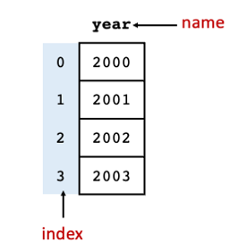
Fig. 3.2 Components of the Series data structure.#
Exercise 3.4 (Exploring DataFrames)
Level:
In this exercise we will be using the dataset from the World Bank Data Catalog that is used in this course. Follow the instructions above to load the dataset into Python and make use of DataFrame methods to answer the following questions:
What type is
df?How many columns and how many rows does the
dfhave?What are the data types of each column?
3.2.7. Slicing DataFrames#
Fig. 3.3 shows the core components of the DataFrame data structure. The first column we see when we look at the
contents of df is the index. The index is a column of data items in the DataFrame but rather it contains the index
positions of each record in the DataFrame. Like all the other data structures in Python we have looked at so far, it
starts with 0.

Fig. 3.3 Components of the DataFrame data structure.#
We can extract columns, rows or data items from DataFrames in different ways. The sections below go over the different ways we can slice DataFrames.
3.2.7.1. Extracting column data (label-based indexing)#
To extract data from a column in the DataFrame we use the following notation:
df[“column_name”]
where df is the DataFrame object. If we want to extract multiple columns, we can provide a Python list of column names
inside the square brackets as follows:
df[[“column_name1”, “column_name2”]]
#extract the column "life_expectancy_t" and save it in variable le_t
le_t = df["life_expectancy_t"]

#check what type is le_t
print(f"Type of le_t is: {type(le_t)}")

# get the length of the Series
print(f"Size of le_t is: {le_t.size}")

#print the first 5 items
le_t.head()
Type of le_t is: <class 'pandas.core.series.Series'>
Size of le_t is: 3038
0    55.841
1    56.308
2    56.784
3    57.271
4    57.772
Name: life_expectancy_t, dtype: float64
Note that in the example above, since we are extracting only one column from df the result of the first slicing is a Series object.
The code below, on the other hand, extracts 3 columns from df, and therefore the result of this is another DataFrame object.
#extract the columns "life_expectancy_t", "life_expectancy_m", "life_expectancy_f" and save it in variable le
le = df[["life_expectancy_t", "life_expectancy_m", "life_expectancy_f"]]

# get type of object returned from slicing
print(f"Type of le is: {type(le)}")

#get size of DataFrame
print(f"Size of le is: {le.shape}")

# print the first 5 items
le.head()
Type of le is: <class 'pandas.core.frame.DataFrame'>
Size of le is: (3038, 3)
| life_expectancy_t | life_expectancy_m | life_expectancy_f | |
|---|---|---|---|
| 0 | 55.841 | 54.663 | 57.120 |
| 1 | 56.308 | 55.119 | 57.596 |
| 2 | 56.784 | 55.583 | 58.080 |
| 3 | 57.271 | 56.056 | 58.578 |
| 4 | 57.772 | 56.542 | 59.093 |
3.2.7.2. Extracting row data (boolean indexing)#
We can extract rows from our DataFrame that meet a specified condition by using the conditional expressions in our slice operators as follows:
df[conditional expression]
Let us try an example on our df DataFrame. We would like to get the records where life expectancy is more than 80:
le_top = df[df["life_expectancy_t"] > 80]
le_top.head()
| country | year | population_m | population_f | population_t | population_density | land_area | life_expectancy_f | life_expectancy_m | life_expectancy_t | co2_emissions_pc | |
|---|---|---|---|---|---|---|---|---|---|---|---|
| 143 | Australia | 2003 | 9926226.0 | 9969174.0 | 19895400.0 | 2.589771 | 7682300.0 | 82.8 | 77.8 | 80.239024 | 17.721684 |
| 144 | Australia | 2004 | 10042276.0 | 10085124.0 | 20127400.0 | 2.619971 | 7682300.0 | 83.0 | 78.1 | 80.490244 | 18.174727 |
| 145 | Australia | 2005 | 10177992.0 | 10216808.0 | 20394800.0 | 2.654778 | 7682300.0 | 83.3 | 78.5 | 80.841463 | 18.146292 |
| 146 | Australia | 2013 | 11541758.0 | 11586371.0 | 23128129.0 | 3.010574 | 7682300.0 | 84.3 | 80.1 | 82.148780 | 16.442316 |
| 147 | Australia | 2014 | 11705167.0 | 11770519.0 | 23475686.0 | 3.055815 | 7682300.0 | 84.4 | 80.3 | 82.300000 | 15.830422 |
Similarly to Numpy, you can combine different comparison expressions using the & (and) or | (or) operators. You would
need to wrap each conditional expression in parentheses. See example below:
# get all records that have life expectancy > 80, where year is either 2020 or 2019
le_top[(le_top["year"] == 2020) | (le_top["year"] == 2019)]
| country | year | population_m | population_f | population_t | population_density | land_area | life_expectancy_f | life_expectancy_m | life_expectancy_t | co2_emissions_pc | |
|---|---|---|---|---|---|---|---|---|---|---|---|
| 152 | Australia | 2019 | 12632259.0 | 12733486.0 | 25365745.0 | 3.297670 | 7692020.000 | 85.0 | 80.9 | 82.900000 | 15.238267 |
| 153 | Australia | 2020 | 12794929.0 | 12898338.0 | 25693267.0 | 3.340250 | 7692020.000 | 85.3 | 81.2 | 83.200000 | NaN |
| 166 | Austria | 2019 | 4372358.0 | 4507562.0 | 8879920.0 | 107.609307 | 82520.000 | 84.2 | 79.7 | 81.895122 | 7.293984 |
| 167 | Austria | 2020 | 4395554.0 | 4521310.0 | 8916864.0 | 108.057004 | 82520.000 | 83.6 | 78.9 | 81.192683 | NaN |
| 264 | Belgium | 2019 | 5686560.0 | 5802420.0 | 11488980.0 | 379.424703 | 30280.000 | 84.3 | 79.8 | 81.995122 | 8.095584 |
| ... | ... | ... | ... | ... | ... | ... | ... | ... | ... | ... | ... |
| 2631 | Sweden | 2020 | 5186267.0 | 5167175.0 | 10353442.0 | 25.420723 | 407283.532 | 84.2 | 80.7 | 82.407317 | NaN |
| 2644 | Switzerland | 2019 | 4252686.0 | 4322594.0 | 8575280.0 | 217.007630 | 39516.030 | 85.8 | 82.1 | 83.904878 | 4.359041 |
| 2645 | Switzerland | 2020 | 4284690.0 | 4351871.0 | 8636561.0 | 218.558418 | 39516.030 | 85.2 | 81.1 | 83.100000 | NaN |
| 2882 | United Kingdom | 2019 | 33008768.0 | 33827559.0 | 66836327.0 | 276.263080 | 241930.000 | 83.1 | 79.4 | 81.204878 | 5.220514 |
| 2883 | United Kingdom | 2020 | 33144663.0 | 33936337.0 | 67081000.0 | 277.274418 | 241930.000 | 82.9 | 79.0 | 80.902439 | NaN |
78 rows × 11 columns
You can write the same code using the isin() function which providing it with a list of values, it returns True for
each row where the values are present. The example below returns the same result as the code above, but it uses the isin()
function to check whether each row in le_top has either 2000 or 2019 in the year column.
le_top[le_top["year"].isin([2020, 2019])]
| country | year | population_m | population_f | population_t | population_density | land_area | life_expectancy_f | life_expectancy_m | life_expectancy_t | co2_emissions_pc | |
|---|---|---|---|---|---|---|---|---|---|---|---|
| 152 | Australia | 2019 | 12632259.0 | 12733486.0 | 25365745.0 | 3.297670 | 7692020.000 | 85.0 | 80.9 | 82.900000 | 15.238267 |
| 153 | Australia | 2020 | 12794929.0 | 12898338.0 | 25693267.0 | 3.340250 | 7692020.000 | 85.3 | 81.2 | 83.200000 | NaN |
| 166 | Austria | 2019 | 4372358.0 | 4507562.0 | 8879920.0 | 107.609307 | 82520.000 | 84.2 | 79.7 | 81.895122 | 7.293984 |
| 167 | Austria | 2020 | 4395554.0 | 4521310.0 | 8916864.0 | 108.057004 | 82520.000 | 83.6 | 78.9 | 81.192683 | NaN |
| 264 | Belgium | 2019 | 5686560.0 | 5802420.0 | 11488980.0 | 379.424703 | 30280.000 | 84.3 | 79.8 | 81.995122 | 8.095584 |
| ... | ... | ... | ... | ... | ... | ... | ... | ... | ... | ... | ... |
| 2631 | Sweden | 2020 | 5186267.0 | 5167175.0 | 10353442.0 | 25.420723 | 407283.532 | 84.2 | 80.7 | 82.407317 | NaN |
| 2644 | Switzerland | 2019 | 4252686.0 | 4322594.0 | 8575280.0 | 217.007630 | 39516.030 | 85.8 | 82.1 | 83.904878 | 4.359041 |
| 2645 | Switzerland | 2020 | 4284690.0 | 4351871.0 | 8636561.0 | 218.558418 | 39516.030 | 85.2 | 81.1 | 83.100000 | NaN |
| 2882 | United Kingdom | 2019 | 33008768.0 | 33827559.0 | 66836327.0 | 276.263080 | 241930.000 | 83.1 | 79.4 | 81.204878 | 5.220514 |
| 2883 | United Kingdom | 2020 | 33144663.0 | 33936337.0 | 67081000.0 | 277.274418 | 241930.000 | 82.9 | 79.0 | 80.902439 | NaN |
78 rows × 11 columns
3.2.7.3. Extracting rows and columns#
To extract rows and columns from a DataFrame we need to use the loc and iloc operators.
3.2.7.3.1. loc#
loc is mainly used with label-based indexing and boolean indexing. The general usage format is the following:
df.loc[row condition expression, column_name]
In the example below we extract the list of countries from our df DataFrame where life expectancy is greater than 80.
countries = df.loc[df["life_expectancy_t"] > 80, "country"]

print(f"Type of countries is: {type(countries)}")
print(f"Length of Series is: {countries.size}")

# use unique method of Series to remove duplicates
print(countries.unique())
Type of countries is: <class 'pandas.core.series.Series'>
Length of Series is: 333
['Australia' 'Austria' 'Belgium' 'Bermuda' 'Canada' 'Channel Islands'
 'Chile' 'Costa Rica' 'Cyprus' 'Denmark' 'Faroe Islands' 'Finland'
 'France' 'Germany' 'Greece' 'Guam' 'Hong Kong SAR, China' 'Iceland'
 'Ireland' 'Israel' 'Italy' 'Japan' 'Korea, Rep.' 'Liechtenstein'
 'Luxembourg' 'Macao SAR, China' 'Malta' 'Netherlands' 'New Zealand'
 'Norway' 'Portugal' 'Puerto Rico' 'Qatar' 'Singapore' 'Slovenia' 'Spain'
 'St. Martin (French part)' 'Sweden' 'Switzerland' 'United Kingdom']
3.2.7.3.2. iloc (integer-based indexing)#
iloc is mainly used with integer-based indexing, which means that index positions are supplied to iloc in the following
format:
df[R, C]
where R is the row index position and C is the column index position. In short, if you want to extract data items from a
DataFrame based on index positions, than iloc is the way to do that.
#get the first 10 rows and the first 5 columns of the df Dataframe
df.iloc[0:10, 0:5]
| country | year | population_m | population_f | population_t | |
|---|---|---|---|---|---|
| 0 | Afghanistan | 2000 | 10689508.0 | 10090449.0 | 20779957.0 |
| 1 | Afghanistan | 2001 | 11117754.0 | 10489238.0 | 21606992.0 |
| 2 | Afghanistan | 2002 | 11642106.0 | 10958668.0 | 22600774.0 |
| 3 | Afghanistan | 2003 | 12214634.0 | 11466237.0 | 23680871.0 |
| 4 | Afghanistan | 2004 | 12763726.0 | 11962963.0 | 24726689.0 |
| 5 | Afghanistan | 2005 | 13239684.0 | 12414590.0 | 25654274.0 |
| 6 | Afghanistan | 2013 | 16554278.0 | 15715314.0 | 32269592.0 |
| 7 | Afghanistan | 2014 | 17138803.0 | 16232001.0 | 33370804.0 |
| 8 | Afghanistan | 2015 | 17686166.0 | 16727437.0 | 34413603.0 |
| 9 | Afghanistan | 2016 | 18186994.0 | 17196034.0 | 35383028.0 |
Exercise 3.5 (Slicing DataFrames)
Level:
Using the df DataFrame created above, write code to perform the following tasks:
Get the first 3 columns of
df.Get the first 3 rows of
df.Get the first row of
df.What are the maximum and minimum values of life expectancy (use life_expectancy_t column)? Which countries have these?
Extract all the data from the United Kingdom and save it into another DataFrame. How many records were returned?
Extract all the records from the United Kingdom from the year 2020. How many records were returned?
When extracting rows from a DataFrame, try not using parentheses between two conditional expressions when using
&or|and see what happens.