3.5. Coupon Collector’s Problem

This section was adapted from Professor Nik Cunniffe’s MCB Notes. If you would like to refer to the material in this section, please cite as follows:

Cunniffe,Nik (2022), Mathematical and Computational Biology Course Notes and Lectures

In this section we will be going over the Coupon Collector’s Problem:

There are \(n\) different types of coupons. You start with no coupons at all, but every day you are given a new coupon at random. It might already be in your collection, or it might be of a type you do not yet have. The quantity of interest is, \(C(n)\), the number of days it takes to collect the full set of \(n\) coupons.

Let us see how we can write this as a Python program.

import numpy as np

def coupon_collector(n):
    """
    This function performs the coupon collector's problem to collect n coupons.
    :param n: Number of coupons to collect.
    :return: The number of trials made until all the coupons have been collected.
    """
    n_remaining = n  # this variable holds the number of remaining coupons to be collected.
    trials = 0  # the variable holds the number of current iterations or trials done.
    # initialise a list of size n with False, each item in the list to represent whether the respective coupon has been
    # collected (True) or not (False)
    coupon_collected = np.full(n, False)
    # repeat until the number of remaining coupons to be collected is 0.
    while n_remaining > 0:
        # generate a random number from 0 to n (excluded)
        coupon_n = rng.integers(low=0, high=n)
        # if current coupon has not been collected before:
        #   collect coupon
        #   and reduce the number of coupons to be collected by 1
        if not coupon_collected[coupon_n]:
            coupon_collected[coupon_n] = True
            n_remaining = n_remaining - 1
        # increase the number of trial by 1
        trials = trials + 1
    # the function will stop when the number of coupons left to be collected is zero
    return trials


# set up random number generator with seed
seed = 62354124
rng = np.random.default_rng(seed)
# perform 200 simulations of the coupon collector problem
iterations = 200
# number of coupons to collect is 100 (n)
coupons = 100
# initialise an array of zeros - 1 item for each coupon collector simulation
c = np.zeros(iterations)

# perform simulations:  in each iteration save the number of trials made to collect all coupons.
for i in range(iterations):
    c[i] = coupon_collector(coupons)

# the expectation on C(n) is the average of all simulations
print(f"Estimated C({coupons}) = {np.average(c):.2f} ({iterations} replicate runs)")

Estimated C(100) = 513.95 (200 replicate runs)

The main point of Monte Carlo method is that when there is something probabilistic that we cannot predict (like the time to collect the whole set of coupons), we need to do a lot of simulations to make sure that we get a close enough accurate estimation. To do this, in the example below we repeat simulations as done above a few times (300 times in the example below).

import matplotlib.pyplot as plt

repeats = 100  # repeat simulations 150 times
c_repeats = np.empty(repeats)  # this array will contain the expected number of trials to collect all coupons for each repeated simulation


for j in range(repeats):
    # print every 10 steps, just as reassurance that something is happening while you wait!
    if j % 10 == 0:
        print(f"Doing small test run {j}")

    c = np.zeros(iterations)
    for i in range(iterations):
        c[i] = coupon_collector(coupons)

    c_repeats[j] = np.average(c)

# plot the simulations in a plot to check distribution
figure, axis = plt.subplots(2,2)

axis[0,0].hist(c_repeats[0:10])
axis[0,0].set_title("10 repeated simulations")
axis[0,1].hist(c_repeats[0:25])
axis[0,1].set_title("50 repeated simulations")
axis[1,0].hist(c_repeats[0:50])
axis[1,0].set_title("100 repeated simulations")
axis[1,1].hist(c_repeats)
axis[1,1].set_title("150 repeated simulations")

#use this to remove overlap of title with axis
figure.tight_layout()

plt.show()

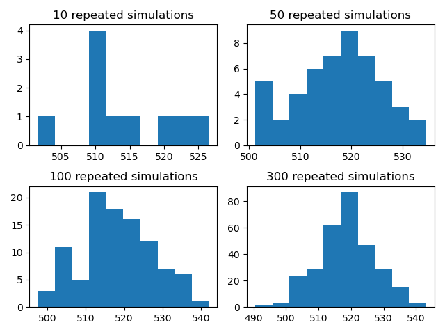
In the plot generated above we can see that the larger the number of repeated simulations, the sample distribution becomes close to that of a normal distribution. This is in line with the central limit theorem.