3.1. Matrices in NumPy

Matrices are used in several fields of study, including, mathematics, computer science and engineering. In this section we will be introducing matrices and the core matrix operations. We will be doing this using NumPy matrices.

3.1.1. Types of Matrices

Let’s start from the very beginning, by looking at different types of matrices.

• A matrix consisting of a single row is called a row matrix.

• A matrix consisting of a single column is called a column matrix. We have already seen this in Practical 2 where we introduced 1-D NumPy arrays or vectors.

• A matrix which has \(n\) rows and \(n\) columns, that is, the same number of rows and columns, is called a square matrix.

• A matrix which has \(n\) rows and \(m\) columns, is called a rectangular matrix.

3.1.2. Creating a NumPy matrix

We create a matrix in NumPy in a similar way we did with a NumPy vector, but using nested lists instead of a list, as follows:

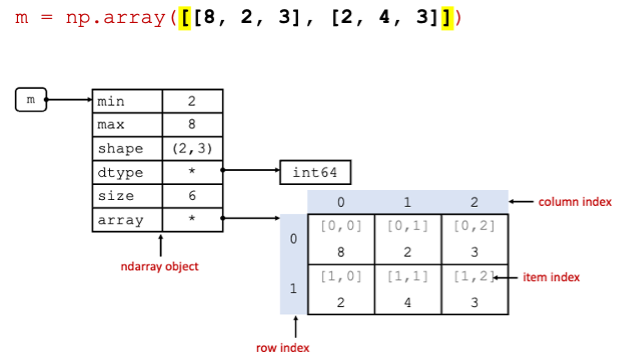
matrix above shows a representation of the ndarray object created in memory after running the code m = np.array([[8, 2, 3], [2, 4, 3]]). In this example, variable m points to an ndarray object in memory. The ndarray object is composed of different attributes. The data of the ndarray object is not stored inside the ndarray object, the ndarray object points to it. The main difference from the 1D NumPy arrays is mainly in the shape attribute, which now stored 2 numbers representing the size of the rows and columns of the matrix respectively.

3.1.3. Matrix products

Most matrix operations are similar to those that we have done in practical 2 for vectors. In this section we look at the dot product multiplication and how to calculate the determinant of a matrix . I have included details on how these are computed mathematically for those who do not have this background or who would like to refresh it. Please skip these explanations and only look at the python code if you are already familiar with this.

3.1.3.1. Dot product multiplication

Assume the following matrices A and B:

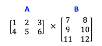
The matrix product \(AB\) is defined only when the number of columns in \(A\) is the same as the number of rows in \(B\).

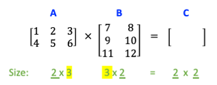
In the matrices above the size of each matrix is defined in green under each matrix. Note that the size of columns in \(A\) is the same as the size of rows in \(B\) (highlighted in yellow). The size of the product is defined by the remaining dimensions underlined in green in the figure above, that is, from the sizes above, we know that the product will be of size \(2 \times 2\).

It is important to note that matrix multiplication is not commutative, that is, \(AB \neq BA\). Below are the steps to perform multiplication of two matrices.

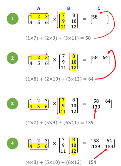
The code to compute \(AB\) above in NumPy is as follows:

import numpy as np

a = np.array([[1, 2, 3], [4, 5, 6]])
b = np.array([[7, 8], [9, 10], [11, 12]])

c = np.dot(a, b)
print(c)

[[ 58  64]
 [139 154]]

3.1.3.2. Determinant of a 2 x 2 matrix

A determinant is a scalar that is calculated from a square matrix as follows:

Given a matrix \(A\):

\[\begin{split} A = \begin{bmatrix} a & b\\ c& d\\ \end{bmatrix} \end{split}\]

The determinant of \(A\) is \(|A|\) where \(|A| = ad-bc\)

Let us try to calculate a determinant of a matrix in the example below.

\[\begin{split} A = \begin{bmatrix} 1 & 4 \\ -1 & -1 \\ \end{bmatrix} \end{split}\]

Using the formula \(|A| = ad-bc\), the determinant of \(A\) can be calculated as:

\[\begin{split} \begin{align} |A| & = (1 \times -1) - (4 \times -1)\\ & = -1 + 4 \\ & = 3 \end{align} \end{split}\]

Using NumPy this is coded as:

a = np.array([[1, 4], [-1, -1]])
det_a = np.linalg.det(a)
print(f"{det_a:.2f}")

3.00

3.1.4. NumPy Matrix manipulation operations

Below is a list of useful NumPy matrix operations. For the examples below we will be using the following matrix:

m = np.array([[8, 2, 3], [2, 3, 4], [4, 8, 9]])

Table 3.1 NumPy matrix manipulation functions

Function	Description	Example
np.delete(m, obj, axis)	obj is the index of the row or column to be deleted. axis is the axis to delete - in a 2D array, the row is axis = 0 and the column is axis = 1. The function returns a new NumPy array with the specified obj removed.	np.delete(m, 0, 1)
np.insert(m, obj, values, axis)	obj is the index before which the row or column is to be inserted. values to insert into arr. axis is the axis along which to insert values in a 2D array, the row is axis = 0 and the column is axis = 1. The function returns a new NumPy array with the values inserted in arr.	np.insert(m, 1, [2, 3, 4], 0)
a.flatten()	Returns a copy of the array flattened into 1D vector.	arr.flatten()
np.unique(m)	returns the unique data items in arr.	np.unique(m)
np.sort(m, axis)	Returns a copy of the matrix sorted. If axis is 0, columns are sorted in ascending order. If axis is 1, rows are sorted in ascending order.	np.sort(m, 0)

Exercise 3.1 (Manipulating NumPy matrices)

Level:

1. Try the examples in Table 3.1. Check the output of each example.

2. Sort each row of NumPy matrix m in descending order.

3. Using NumPy matrix m:

   a. Get the frequency of each value in the array.
   b. Get the index positions of the first occurring unique values in the array.

3.1.5. Slicing NumPy Matrices

Similarly to NumPy 1D vectors, we slice a NumPy matrix when we want to extract data items from it. The image below shows a few examples of NumPy array slicing:

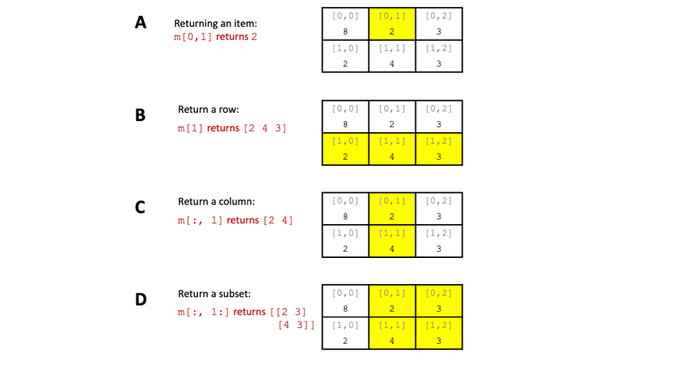
Fig. 3.1 Different examples of matrix slicing using the matrix m = np.array([[8, 2, 3], [2, 4, 3]])

Exercise 3.2 (Shaping a matrix)

Level:

Create a NumPy matrix m of shape 2, 4 by generating 8 integers and then shaping the matrix to the desired size.

Exercise 3.3 (sum of matrix columns)

Level:

Using the matrix m created above, calculate the sum of columns of m

calculate sum of each column in a matrix: print the sum of each column of m_rand