More Pandas
Contents
3.4. More Pandas#
3.4.1. Create a new column#
Similar to NumPy, Pandas supports vectorised operations. This means, that we do not need to create loops to
perform basic element-wise operations. In the example below, we create a new column population_p, that takes the values
of column population_t and divides them by the values of column land_area.
import pandas as pd

# read data from file
df = pd.read_csv("data/world-bank-1_data.csv")

# check the size of the DataFrame
print(df.shape)

# calculate the population density
df["population_d"] = df["population_t"]/df["land_area"]

# check the size of the DataFrame again
print(df.shape)

# check the first few rows
df.head()
(3038, 11)
(3038, 12)
| country | year | population_m | population_f | population_t | population_density | land_area | life_expectancy_f | life_expectancy_m | life_expectancy_t | co2_emissions_pc | population_d | |
|---|---|---|---|---|---|---|---|---|---|---|---|---|
| 0 | Afghanistan | 2000 | 10689508.0 | 10090449.0 | 20779957.0 | 31.859861 | 652230.0 | 57.120 | 54.663 | 55.841 | 0.036574 | 31.859861 |
| 1 | Afghanistan | 2001 | 11117754.0 | 10489238.0 | 21606992.0 | 33.127872 | 652230.0 | 57.596 | 55.119 | 56.308 | 0.033785 | 33.127872 |
| 2 | Afghanistan | 2002 | 11642106.0 | 10958668.0 | 22600774.0 | 34.651540 | 652230.0 | 58.080 | 55.583 | 56.784 | 0.045574 | 34.651540 |
| 3 | Afghanistan | 2003 | 12214634.0 | 11466237.0 | 23680871.0 | 36.307546 | 652230.0 | 58.578 | 56.056 | 57.271 | 0.051518 | 36.307546 |
| 4 | Afghanistan | 2004 | 12763726.0 | 11962963.0 | 24726689.0 | 37.910996 | 652230.0 | 59.093 | 56.542 | 57.772 | 0.041655 | 37.910996 |
Similarly, other mathematical operators can be used to perform other arithmethic operations on columns.
Exercise 3.8 (Create columns)
Level:
Using the df DataFrame object created above, create the following new columns:
fraction of male population (population_m_f)
fraction of female population (population_f_f)
3.4.2. Writing data to files#
Now that we have made changes to our dataset, let us save it in a file so that we keep it safe. To save our dataset into a
.csv format the to_csv() method is used.
df.to_csv("data/world-bank-1m_data.csv")
In the code above, the to_csv()method is saving the data that is currently present in df into a file called world-bank-1m_data.csv
in the data folder. There are other file formats that DataFrames can be saved into. They normally have the format of to_*. Look
into Pandas documentation for a whole list.
Exercise 3.9 (Saving data into files)
Level:
Perform the following:
Save the
dfDataFrame into a tab-delimited .txt file in the data folder with the name world-bank-1_data.txt.Check the file has been created and open it to verify that it is tab-delimited.
Read the file back into Python into a new DataFrame object (df2) and check that the data has loaded well.
3.4.3. Handling missing data#
Missing data in Pandas is displayed as nan. In practice, if we are compiling a dataset ourselves, we should keep the
respective data item empty so that the dataset can be used by different programming languages and systems.
One useful operation is to remove all rows that have an nan in them (even if it is just in one column). This can be done
by using the dropna() method.
print(f"Size of df is: {df.shape}")

df_complete = df.dropna()

print(f"Size of df_complete is: {df_complete.shape}")
Size of df is: (3038, 12)
Size of df_complete is: (2346, 12)
When dealing with data something you might also want to detect missing values in a column rather than the whole dataset.
The isna() function returns a Series of True and False depending on whether the data item in the Series is nan or not.
The notna() function does the opposite of isna(), it returns False if the respective data item in the Series is nan, and
True if a value is present.
# Aruba does not seems to have co2 emissions data
aruba_data = df[df["country"] == "Aruba"]

co2_emissions_isna = pd.isna(aruba_data["co2_emissions_pc"])
print(co2_emissions_isna)

co2_emissions_notna = pd.notna(aruba_data["co2_emissions_pc"])
print(co2_emissions_notna)
126    True
127    True
128    True
129    True
130    True
131    True
132    True
133    True
134    True
135    True
136    True
137    True
138    True
139    True
Name: co2_emissions_pc, dtype: bool
126    False
127    False
128    False
129    False
130    False
131    False
132    False
133    False
134    False
135    False
136    False
137    False
138    False
139    False
Name: co2_emissions_pc, dtype: bool
3.4.4. Select-Apply-Combine#
So far we have applied operations over all the DataFrame object. However, in data analysis, especially when dealing with big data, a common approach to data exploration is the split-apply-combine strategy. The idea behind this strategy is to split the data into more managable pieces, apply any operations required on the data independently on each piece and then combine the results together. The Fig. 3.4 below illustrates the approach that is done in the split-apply-combine approach.
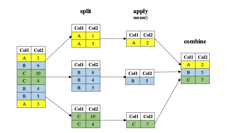
Fig. 3.4 An illustration on how the Split-Apply-Combine strategy works.#
The code below is the Python version of the Split-Apply-Combine approach. In this code, we are splitting the df DataFrame
by year. For each year records, we are applying the mean() function on it. We are the combining the results from each year grouping
and merging it into one DataFrame which is then stored in the res variable.
# for each year, get the average co2 emissions
res = df.groupby("year")["co2_emissions_pc"].mean()
print(res)
year
2000    4.244367
2001    4.323111
2002    4.349692
2003    4.466854
2004    4.505477
2005    4.525854
2013    4.326678
2014    4.226973
2015    4.184129
2016    4.195432
2017    4.199802
2018    4.164970
2019    4.115138
2020         NaN
Name: co2_emissions_pc, dtype: float64
Exercise 3.10 (Select-Apply-Combine)
Level:
Find the maximum value of CO2 emmissions for each country in the df DataFrame.
Exercise 3.11 (Becoming an independent programmer)
Level:
The purpose of this course is to teach you the core concepts well. It is up to you to then apply these concepts to solve your computational/mathematical problems.
One thing you should be aware of is that popular packages normally have a cheat sheet. A cheat sheet is a summarised but user-friendly version of all the functionality of a package. You can find the cheat sheet for pandas here and Matplotlib here.
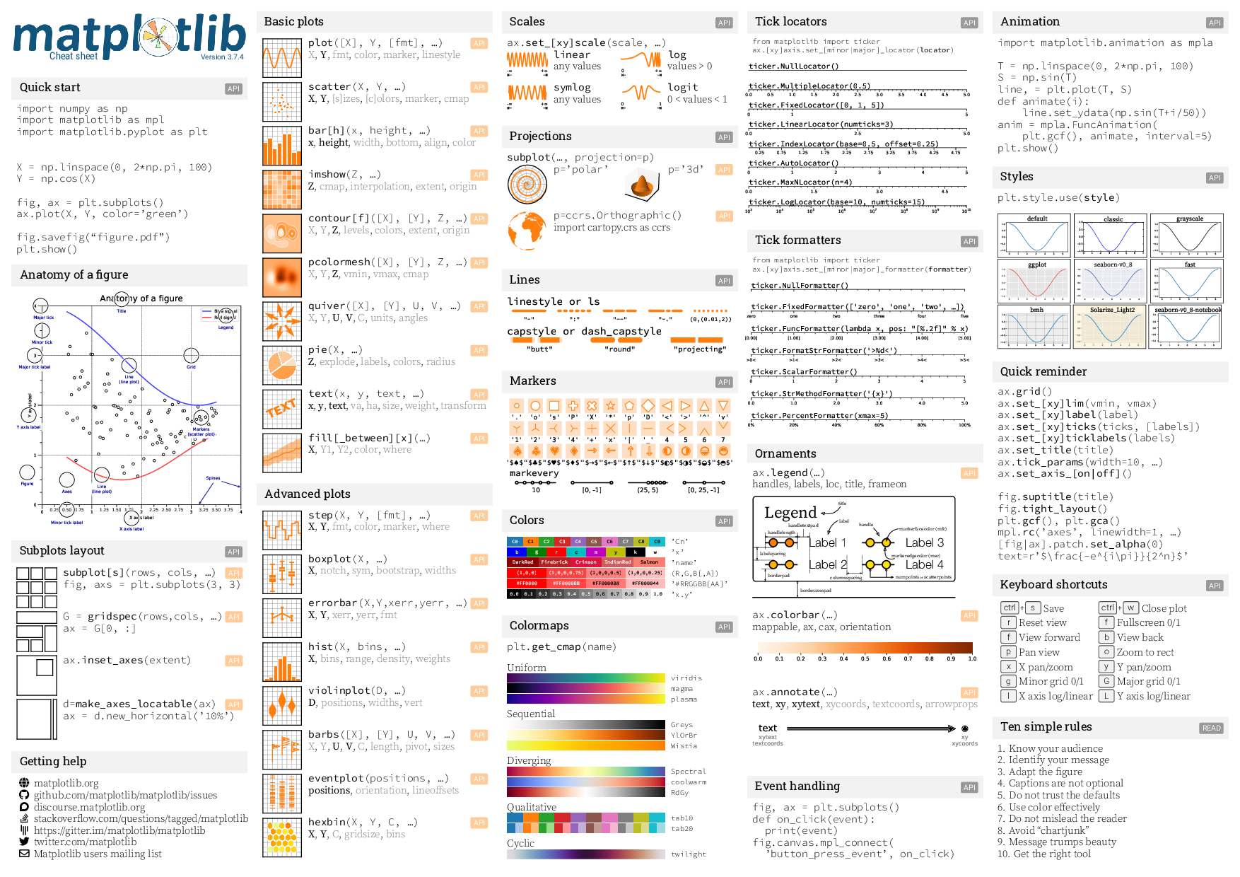
Have a look at the cheat sheet and attempt using a new functionality.
Note
The cheat sheet alone is not enough. To maximise your potential as a programmer you would also need to use the reference documentation
of each respective package. If you go in the documentation of a function and scroll down to the bottom of the page, you will also see
exercises that will help you understand better (the sometimes complex) documentation.
Link to Matplotlib documentation.
Link to Pandas documentation
Use the links above to explore the documentation of Matplotlib and Pandas.