#sort weight in ascending order
surveys_complete %>%
arrange(weight)5 Further data manipulation and visualisation with tidyverse
5.1 Sorting data
To sort your data dplyr provides function arrange.
To sort your data in descending order you will need to use desc().
#sort weight in descending order
surveys_complete %>%
  arrange(desc(weight))
You can sort your dataset based on the values of multiple columns:
#sort weight in ascending order and hindfoot_length in descending order
surveys_complete %>%
  arrange(weight, desc(hindfoot_length))
As you can see from the result returned, the animals with the smallest weight are at the top. When there is a tie, i.e., more than one animal has the same weight, the animals are sorted in descending order of hindfoot_length. As you can see, the subset of animals with weight of 4 have been sorted in descending order based on hindfoot_length.
5.2 Summarising data
Creating summaries of your data would be a good way to start describing the variable you are working with. Summary statistics are a good example of how one can summarise data. We will not cover details about summary statistics in this course, but we will look at how we can summarise data in R. When working with continuous variables, one of the most popular summary statistic is the mean. If we try to calculate the mean on weight in the surveys_complete dataset we get:
surveys_complete %>%
  mean_weight = mean(weight)
Error in mean(weight): object 'weight' not foundThis is because in dplyr you will need to use the summarise function to be able to create summaries of your data.
5.2.1 Frequency - count
Obtaining the frequency of your data is another common way of summarising data. Frequencies are normally calculated when working with discrete variables that have a finite number of values, such as categorical data. In our surveys_complete dataset, let us obtain the frequecies of male and female animals present. We can do this by counting the number of “M” and “F” present in the dataset. To do this use the dplyr function count as follows:
  surveys_complete %>%
    count(sex)
# A tibble: 2 × 2
sex n
<chr> <int>
1 F 14584
2 M 16092As you can see count has grouped the categories present in the sex column and returned the frequency of each category. If we wanted to count combination of factors, such as sex and species, we would specify the first and the second factor as the arguments of count():
surveys_complete %>%
  count(sex, species)
# A tibble: 41 × 3
sex species n
<chr> <chr> <int>
1 F albigula 606
2 F baileyi 1617
3 F eremicus 539
4 F flavus 711
5 F fulvescens 55
6 F fulviventer 15
7 F hispidus 91
8 F leucogaster 436
9 F leucopus 16
10 F maniculatus 354
# … with 31 more rows
Exercise 11
Level: 
Using the
surveys_completevariable, how many animals were observed in eachplot_typesurveyed?What is the frequency of each species of each sex observed? Sort each species in descending order of frequency.
5.3 Plotting time series data - geom_line()
Now that we know how to obtain frequencies, let us create a time series plot with ggplot. A time series plot displays values over time with the aim to show how data changes over time. Let us plot years on the x-axis and the frequencies of the yearly observations per genus on the y-axis.
First we need to get the frequencies of the yearly observations per genus:
yearly_counts <- surveys_complete %>%
  count(year, genus)
yearly_counts now contains the following results:
# A tibble: 199 × 3
    year genus               n
   <dbl> <chr>           <int>
 1  1977 Chaetodipus         3
 2  1977 Dipodomys         222
 3  1977 Onychomys           3
 4  1977 Perognathus        22
 5  1977 Peromyscus          2
 6  1977 Reithrodontomys     2
 7  1978 Chaetodipus        23
 8  1978 Dipodomys         629
 9  1978 Neotoma            23
10  1978 Onychomys          80
# … with 189 more rows
Let us plot this in a line plot:
ggplot(data = yearly_counts, mapping = aes(x = year, y = n)) +
     geom_line()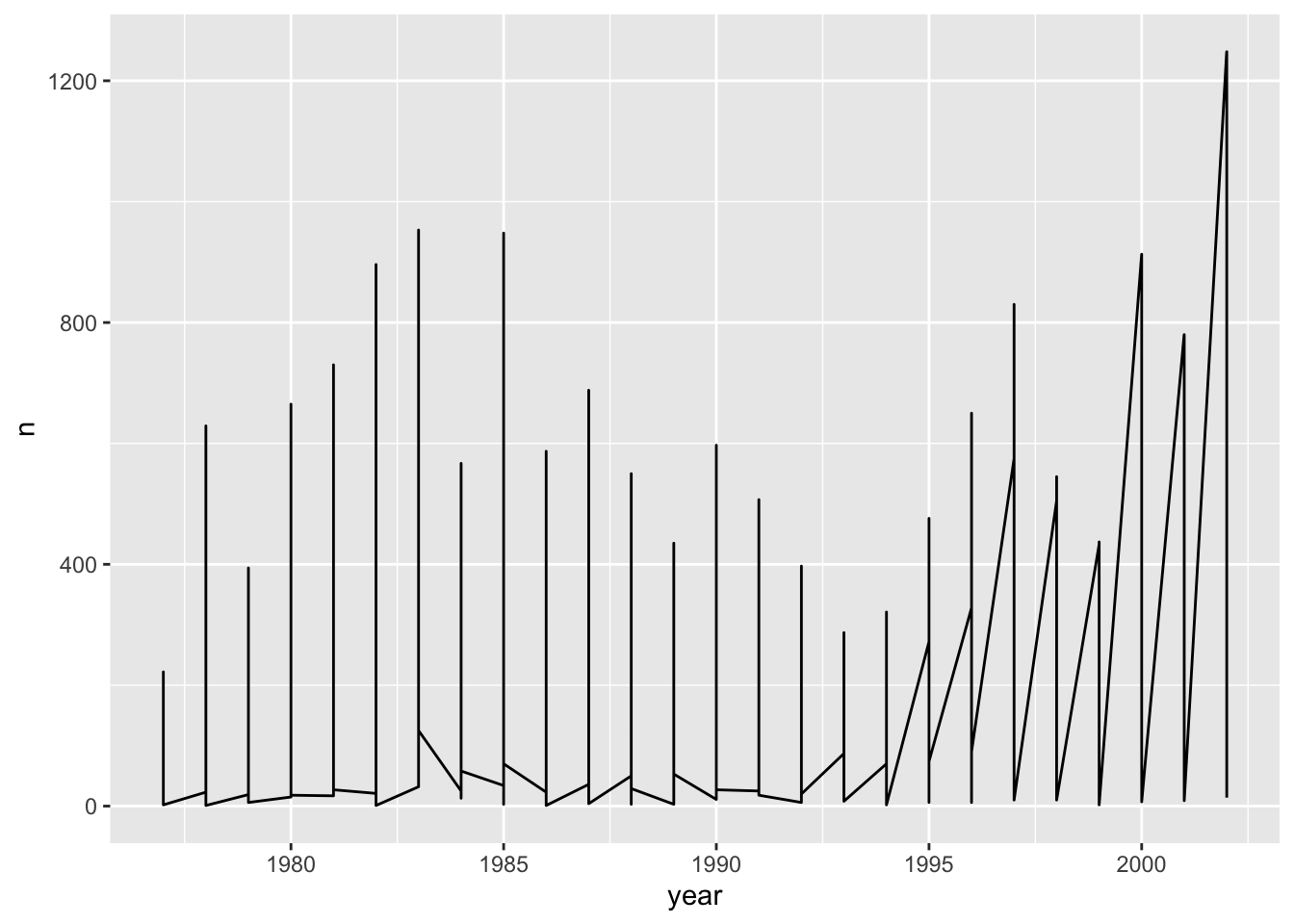
Unfortunately, this does not work because `ggplot plotted data for all the genera together. We need to tell ggplot to draw a line for each genus by modifying the aesthetic function to include group = genus:
ggplot(data = yearly_counts, mapping = aes(x = year, y = n, group = genus)) +
    geom_line()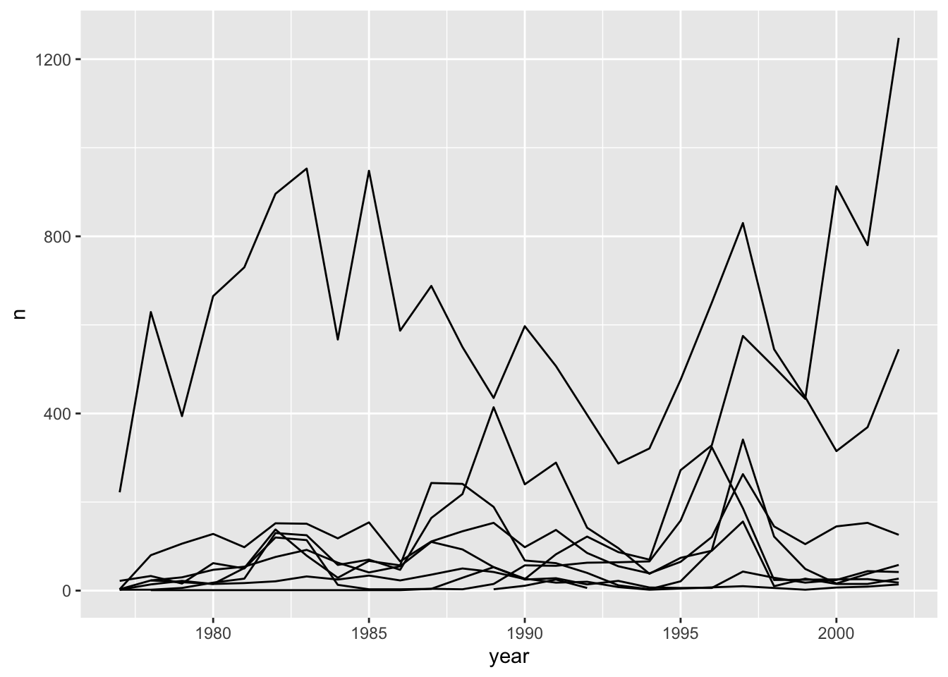
This creates a line for each genus. However, since they are all in the same colour we are not able to distinguish which genus is which. If we use a different colour for each genus the plot should be clear. This is done by using the argument color in the aesthetic function (using color also automatically groups the data):
ggplot(data = yearly_counts, mapping = aes(x = year, y = n, color = genus)) +
    geom_line()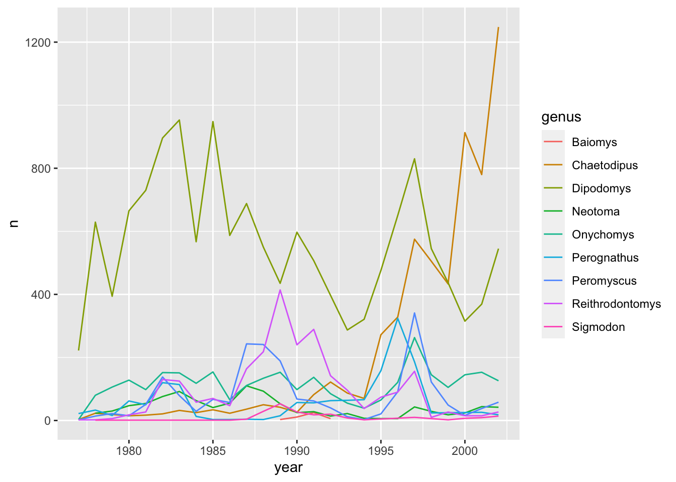
5.4 Plotting single continuous variables - histograms
If you would like to plot the distribution of a single continuous variable the frequency will be automatically calculated, so you do not need to use count() to calculate the frequency beforehand. Histograms are one of the most popular ways to do this. In a histogram, the x-axis is automatically divided into bins and the number of observations of the continuous variable in each bin is shown as a bar in the histogram. In the ggplot2 package a histogram can be plotted using the geom_histogram function.
Let us plot a histogram for the continuous variable weight:
ggplot(surveys_complete, aes(weight)) +
  geom_histogram()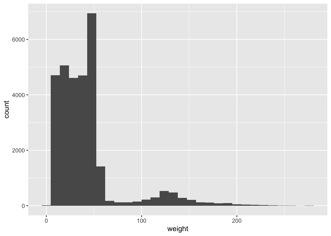
You can identify display categories in the histogram by plotting a stacked histogram which will show categories for each group stacked on top of each other. This is done by using the fill argument in the aesthetic function. If we want to display sex in our weight histogram:
ggplot(surveys_complete, aes(weight, fill=sex)) +
  geom_histogram(bins=100)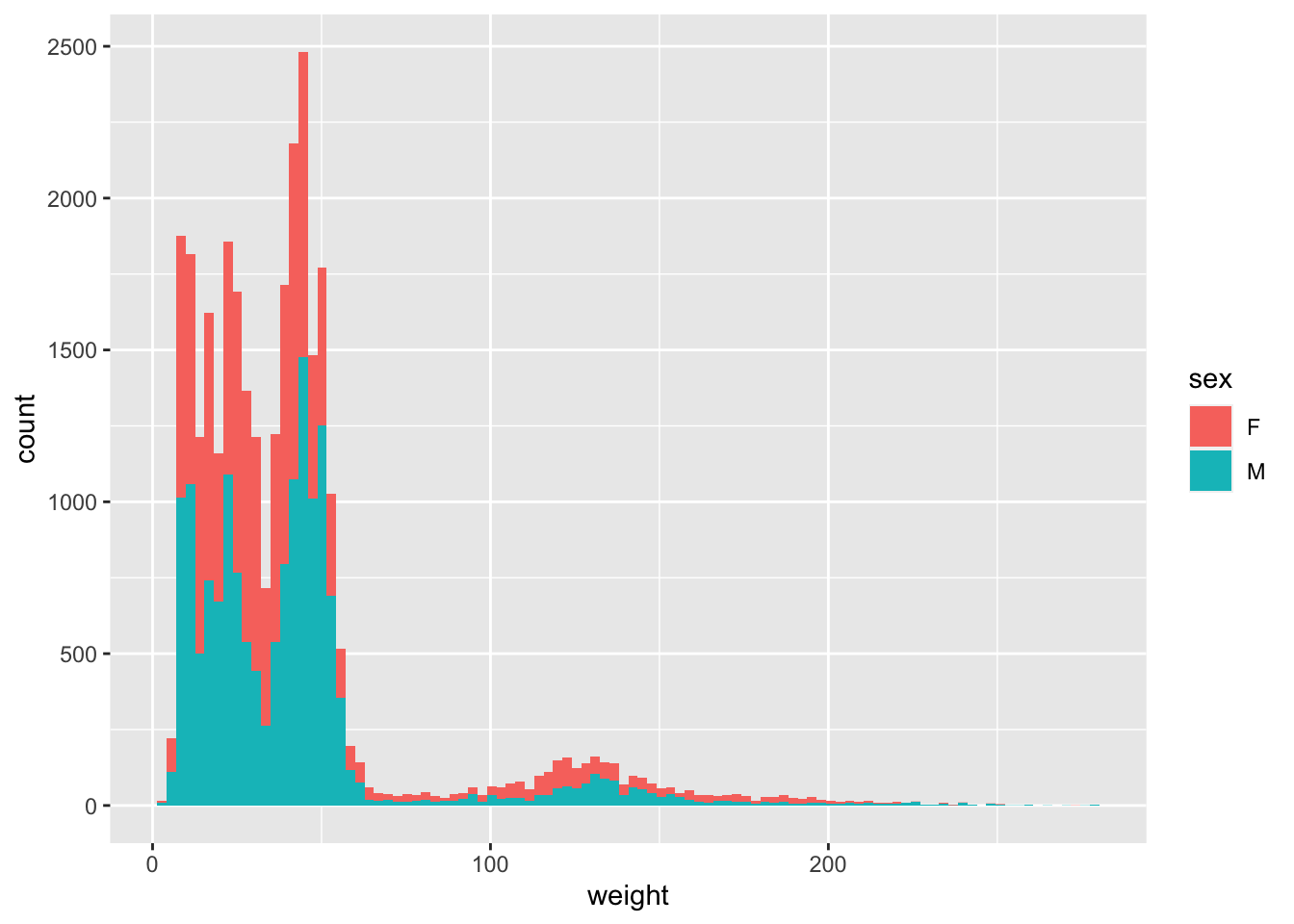
Note that the default number of bins in a histogram is 30. To get a more granular display you can increase the number of bins by using the argument bins in the geom_histogram function as above.
There are other plots that can be used for a single continuous variable (see ONE VARIABLE continuous section on ggplot2 cheat sheet).
Exercise 12
Level: 
Use the geom_freqpoly() to display frequency polygons instead of bars for the distribution of weight. Show sex category as before in a different colour.
Hint
Use the argument color in the aesthetic function rather than fill to display a frequency polygon for each sex category in a different colour.
Solution for Exercise 12
ggplot(surveys_complete, aes(weight, color=sex)) +
  geom_freqpoly()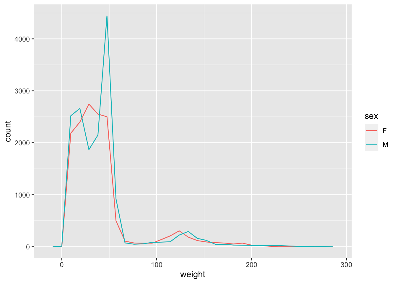
5.5 Grouping data
In the examples above we learnt how to summarise data over all observations, e.g., we calculated the mean over all observations using the summarise function. However, in data analysis, especially when dealing with big data, a common approach to data exploration is the split-apply-combine strategy. The idea behind this strategy is to split the data into more manageable pieces, apply any operations required on the data independently on each piece and then combine the results together. The figure below illustrates the approach that is done in the split-apply-combine approach.

Let us work on an example on how we can apply the split-apply-combine strategy on the surveys_complete dataset. We would like to split the data by the different categories present in the sex column and calculate the mean weight for each category. We can do this as follows:
surveys_complete %>%
  #extract females
  filter(sex=="F") %>%
  summarise(mean_weight = mean(weight))
# A tibble: 1 × 1
mean_weight
<dbl>
1 41.5surveys_complete %>%
#extract males
filter(sex=="M") %>%
summarise(mean_weight = mean(weight))# A tibble: 1 × 1
mean_weight
<dbl>
1 42.1However, this would be a very tedious process to do if we had several categories. We can do this easily by using the group_by function in the dplyr package:
surveys_complete %>%
  group_by(sex) %>%
  summarise(mean_weight=mean(weight))
# A tibble: 2 × 2
sex mean_weight
<chr> <dbl>
1 F 41.5
2 M 42.1You can also group by multiple columns:
surveys_complete %>%
  group_by(sex, species_id) %>%
  summarize(mean_weight = mean(weight))
`summarise()` has grouped output by 'sex'. You can override using the `.groups`
argument.# A tibble: 46 × 3
# Groups: sex [2]
sex species_id mean_weight
<chr> <chr> <dbl>
1 F BA 9.16
2 F DM 41.6
3 F DO 48.5
4 F DS 117.
5 F NL 154.
6 F OL 30.8
7 F OT 24.8
8 F OX 22
9 F PB 30.2
10 F PE 22.8
# … with 36 more rowsOnce the data are grouped, you can also summarize multiple variables at the same time (and not necessarily on the same variable). For instance, we could add a column indicating the minimum weight for each species for each sex:
surveys_complete %>%
  group_by(sex, species_id) %>%
  summarize(mean_weight = mean(weight),
            min_weight = min(weight))
`summarise()` has grouped output by 'sex'. You can override using the `.groups`
argument.# A tibble: 46 × 4
# Groups: sex [2]
sex species_id mean_weight min_weight
<chr> <chr> <dbl> <dbl>
1 F BA 9.16 6
2 F DM 41.6 10
3 F DO 48.5 12
4 F DS 117. 45
5 F NL 154. 32
6 F OL 30.8 10
7 F OT 24.8 5
8 F OX 22 22
9 F PB 30.2 12
10 F PE 22.8 11
# … with 36 more rows
Exercise 13
Level: 
Use
group_by()andsummarise()to find themean,min,maxhind foot length for each species (usingspecies_id) and the number of observations for each species (hint: look into functionn()).What was the heaviest animal measured in each year? Return the columns
year,genus,species, andweight.
5.6 Further visualisations
5.6.1 Facetting
The ggplot2 package has a way of creating different plots based on the different categories in the data. This is known as facetting. With facetting we do not need to use group_by() to split the data into different groups to be able to plot the different categories in different plots as ggplot2 does this automatically.
There are two types of facet functions:
facet_wrap()arranges the different plots into multiple rows and columns to cleanly fit on one page.facet_grid()plots all the categories in 1 row or 1 column.
Let us see this in action. When we plotted a time series plot, we created a line for each different genus. Given there are several genera, it would be more clearer if we plotted each line is a separate plot, one plot for each genus. Facetting will do this very easily. Let us start with facet_wrap(). We supply the variable that we would like to group upon within vars() as following:
ggplot(data = yearly_counts, mapping = aes(x = year, y = n)) +
    geom_line() +
    facet_wrap(facets = vars(genus))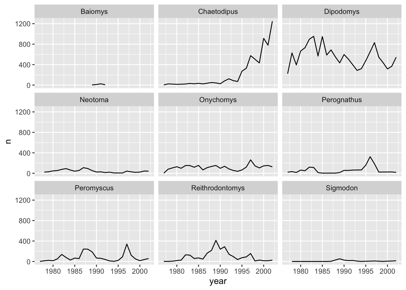
As you can see, each genus has been plotted as a separate plot. It is now clear which are the genera that were observed the most. Another advantage of facetting is that it uses a common axes and all plots are aligned to the same values on the axes, making the different plots comparable. If you want to have different axes for each plot you can do so by using the scales argument.
ggplot(data = yearly_counts, mapping = aes(x = year, y = n)) +
    geom_line() +
    facet_wrap(facets = vars(genus), scales="free")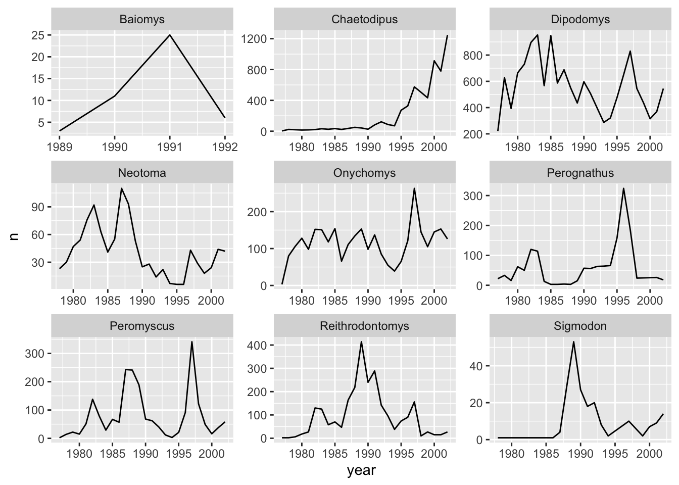
The pattern of the graphs that before were hardly visible, e.g., Baiomys, is now clear as the axes have been rescaled to fit the data. This is the main advantage of using free scales. The disadvantage is that the different plots are not comparable as before.
If we would like to check if there is any difference between the sex, we can do this by adding sex as another grouping to count().
yearly_sex_counts <- surveys_complete %>%
                      count(year, genus, sex)
yearly_sex_counts will now look like:
# A tibble: 389 × 4
    year genus           sex       n
   <dbl> <chr>           <chr> <int>
 1  1977 Chaetodipus     F         3
 2  1977 Dipodomys       F       103
 3  1977 Dipodomys       M       119
 4  1977 Onychomys       F         2
 5  1977 Onychomys       M         1
 6  1977 Perognathus     F        14
 7  1977 Perognathus     M         8
 8  1977 Peromyscus      M         2
 9  1977 Reithrodontomys F         1
10  1977 Reithrodontomys M         1
# … with 379 more rows
This should now allow us to also visualise the same data for the different sex categories. We can use colour to distinguish between the sex categories:
ggplot(data = yearly_sex_counts, mapping = aes(x = year, y = n, color = sex)) +
  geom_line() +
  facet_wrap(facets = vars(genus))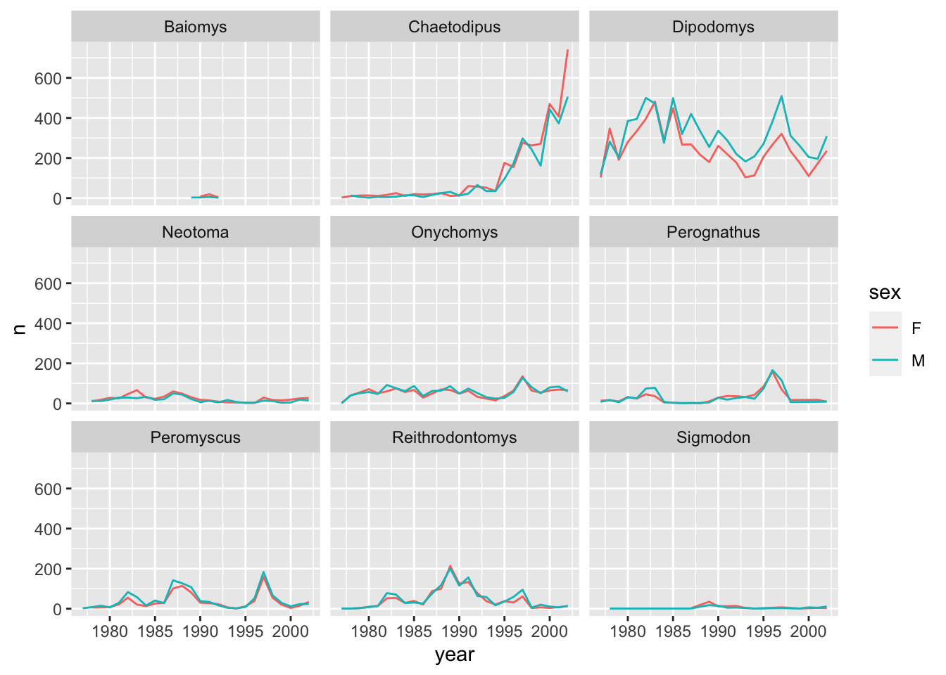
Let us do the same thing with facet_grid() so that we can understand the difference between the two facetting techniques in the ggplot2 package. With facet_grid() you specify what variable you would like to split on as in the rows or cols arguments:
ggplot(data = yearly_counts, mapping = aes(x = year, y = n)) +
    geom_line() +
    #display the genera as columns
    facet_grid(cols = vars(genus))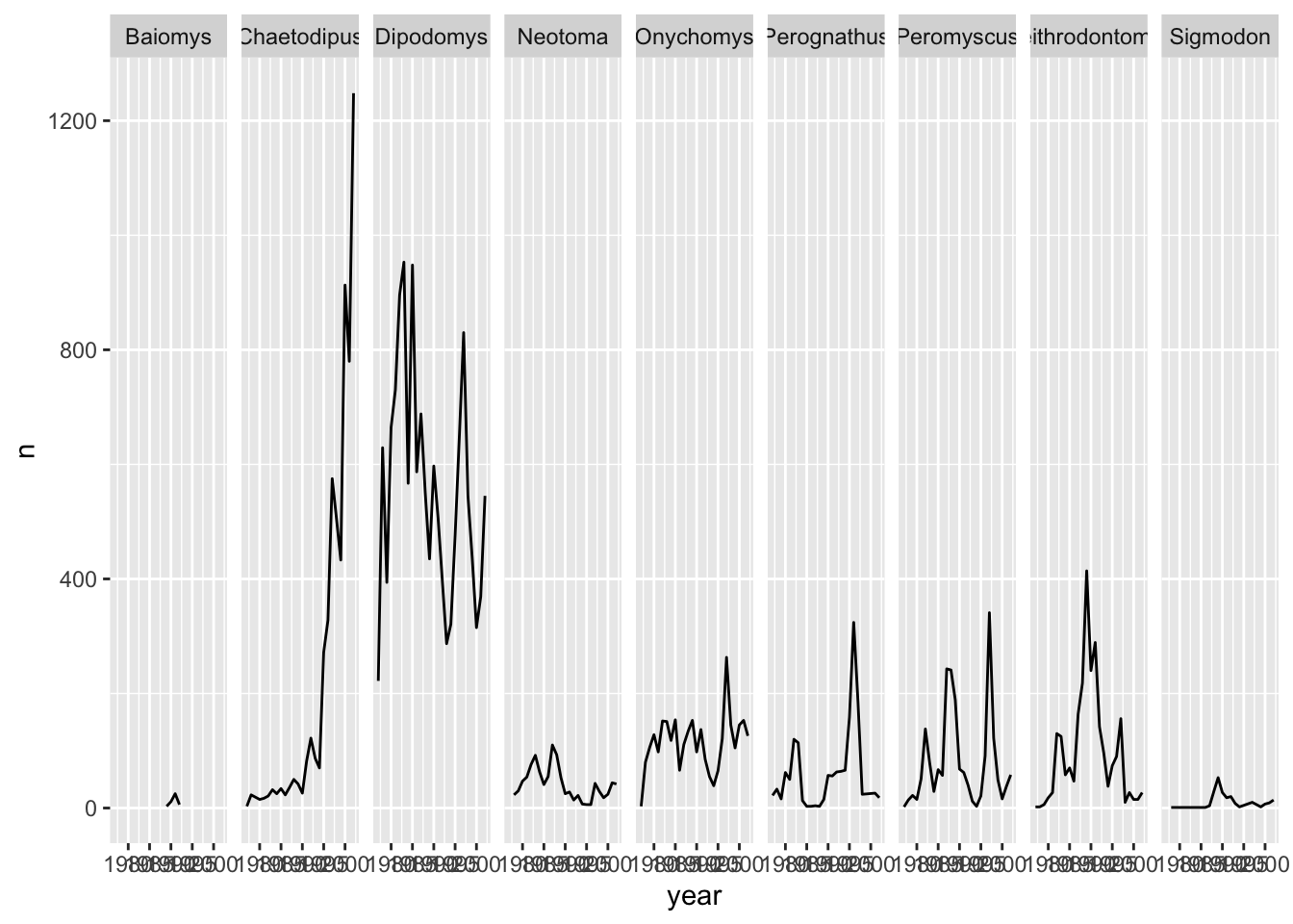
As you can see facet_grid() placed all the categories of genus in 1 row, unlike facet_wrap() which have spread them over multiple rows to fit well in 1 page. Let us split the plots by sex as well by plotting sex as the rows:
ggplot(data = yearly_sex_counts,
  mapping = aes(x = year, y = n)) +
  geom_line() +
  facet_grid(rows = vars(sex), cols =  vars(genus))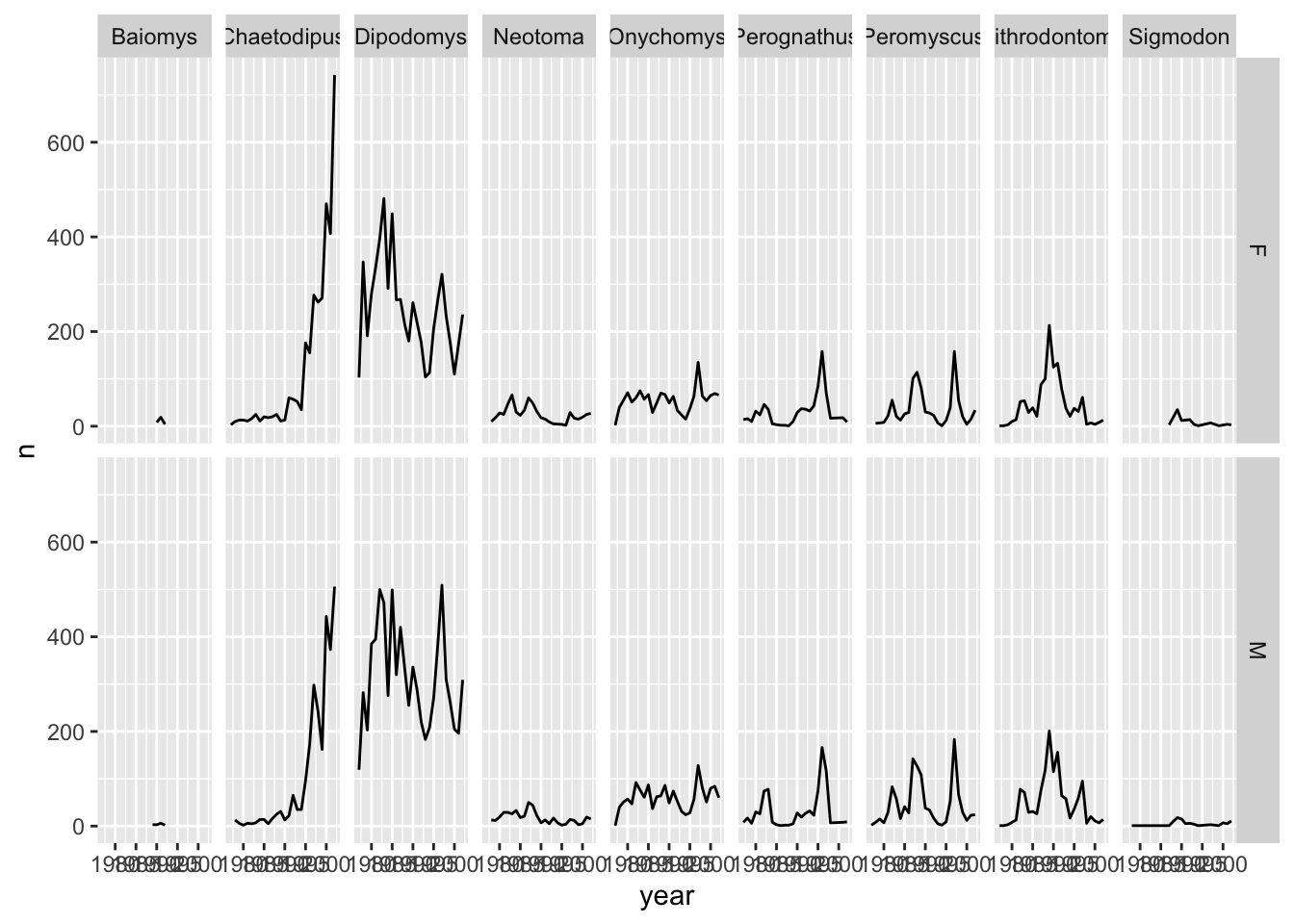
More information on further functionality of facetting can be found in the
facet_wrap()andfacet_grid()documentation.
Exercise 14
Level:
Using the yearly_sex_counts variable above, but instead of splitting the plots by sex as above, draw the frequency of each genus as in here and display the sex as different coloured line graphs in the same plot.
Solution for Exercise 14
ggplot(data = yearly_sex_counts,
  mapping = aes(x = year, y = n, color=sex)) +
  geom_line() +
  facet_grid(cols = vars(genus))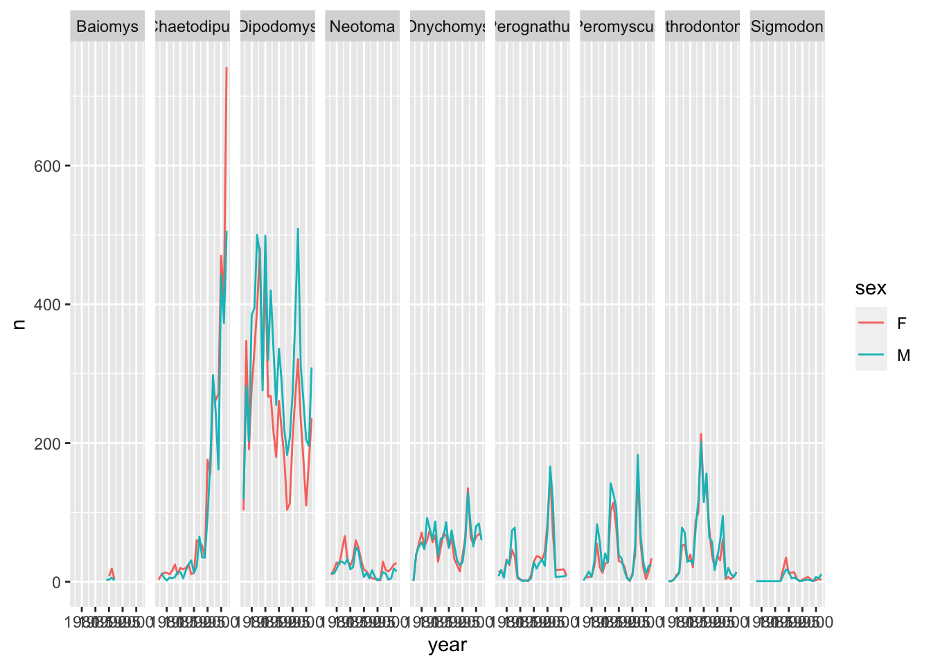
5.6.2 Customisation
Though the default visualisation of ggplot2 plots is already at a good standard, there are several ways one can improve ggplot2 visualisations for publications.
5.6.2.1 Labels
Let us start customising the last plot we have plotted by renaming the axes and adding a title to the plot. This is done by using the labs function:
ggplot(data = yearly_sex_counts, mapping = aes(x = year, y = n)) +
  geom_line() +
  facet_grid(cols = vars(genus)) +
  labs(title = "Observed genera through time",
       x = "Year of observation",
       y = "Number of animals")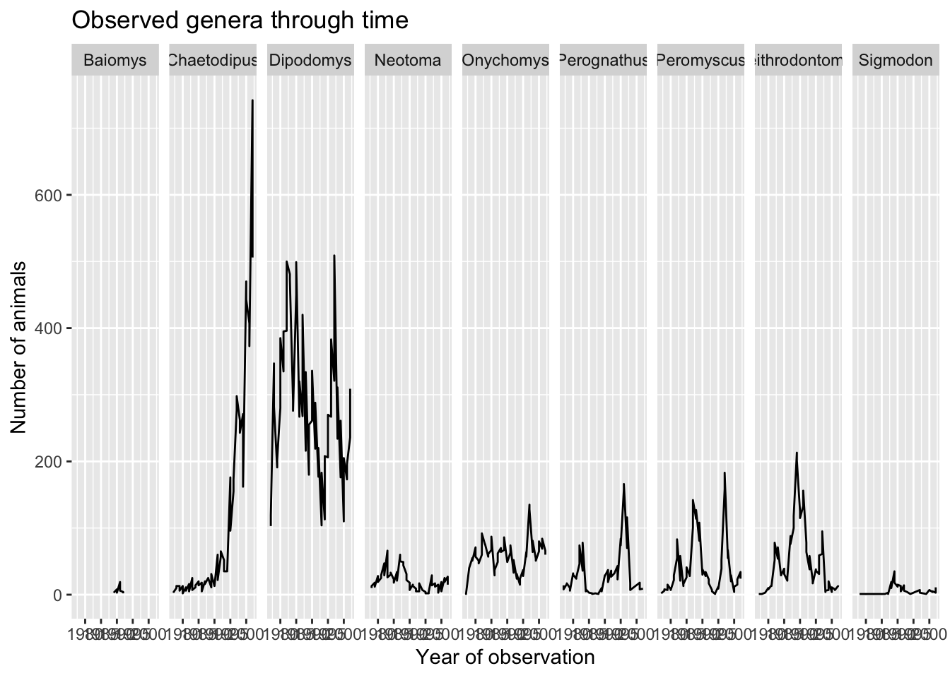
The major item that needs fixing in the plot is the text on the x-axis as this is crammed and is not readable at the moment. This is mainly due to the fact that the size of the plot is dependent on the size of the window (in this case RStudio). You can work around this by saving your plot to a file and specifying the width of the plot (see Saving a plot to a file section). Themes in the ggplot2 package control the display of all non-data elements of the plot. Let us start customising the text on the x-axis by changing its size and position using the theme function. Note that theme() has several other arguments and you can read more about them in the theme() documentation.
ggplot(data = yearly_sex_counts, mapping = aes(x = year, y = n, color=sex)) +
    geom_line() +
    facet_grid(cols = vars(genus)) +
    labs(title = "Observed genera through time",
         x = "Year of observation",
         y = "Number of animals")  +
    theme(axis.text.x = element_text(size=7, angle=90, vjust=0.5),
          axis.text.y = element_text(size=7),
          strip.text=element_text(size=7, angle=45))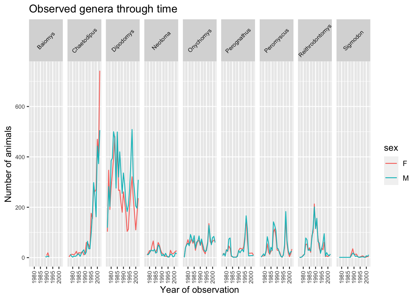
5.6.2.2 Legend
With the plot already looking better, the last thing we would like to change is the legend. Legends are very tricky in ggplot2 as the function to use is determined by the data that is being displayed. In this case the legend has been created based on color groupings. Therefore we can change the legend title, categories and colour as follows:
ggplot(data = yearly_sex_counts, mapping = aes(x = year, y = n, color=sex)) +
    geom_line() +
    facet_grid(cols = vars(genus)) +
    labs(title = "Observed genera through time",
         x = "Year of observation",
         y = "Number of animals")  +
    theme(axis.text.x = element_text(size=7, angle=90, vjust=0.5),
          axis.text.y = element_text(size=7),
          strip.text=element_text(size=7, angle=45)) +
    scale_color_brewer("Sex",
                       palette="Set1",
                       breaks=c("F", "M"),
                       labels=c("Female", "Male"))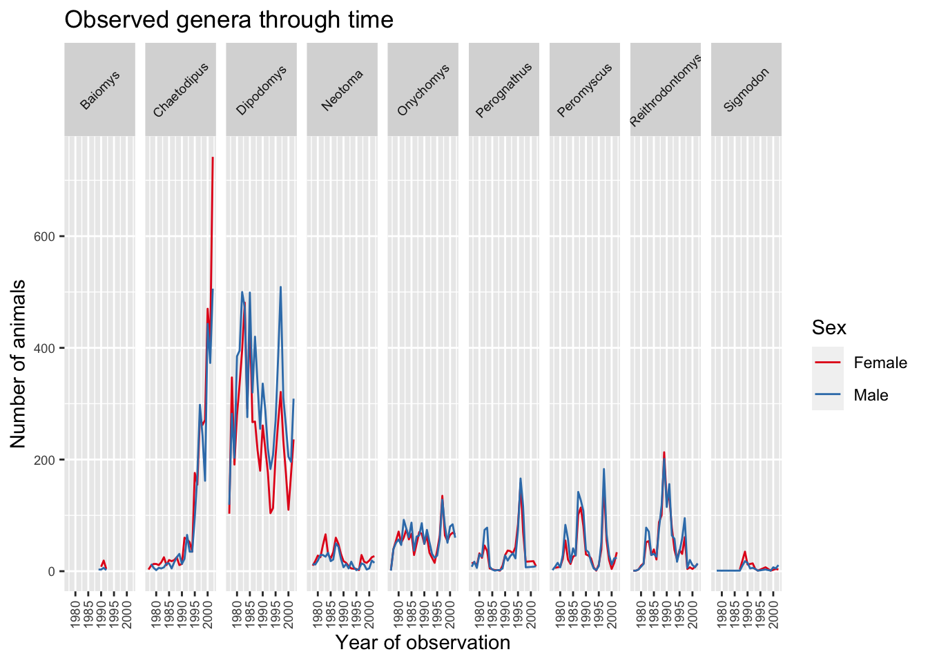
Note
If you would like to see what other palettes are available please have a look at this colour brewer website.
5.6.2.3 Themes
ggplot2 has a set of themes that can be used to change the overall appearance of the plot without much effort. For example, if we create the first plot again and apply the theme_bw() theme we get a more simpler white background:
ggplot(data = surveys, mapping = aes(x = weight, y = hindfoot_length)) +
  geom_point() +
  theme_bw()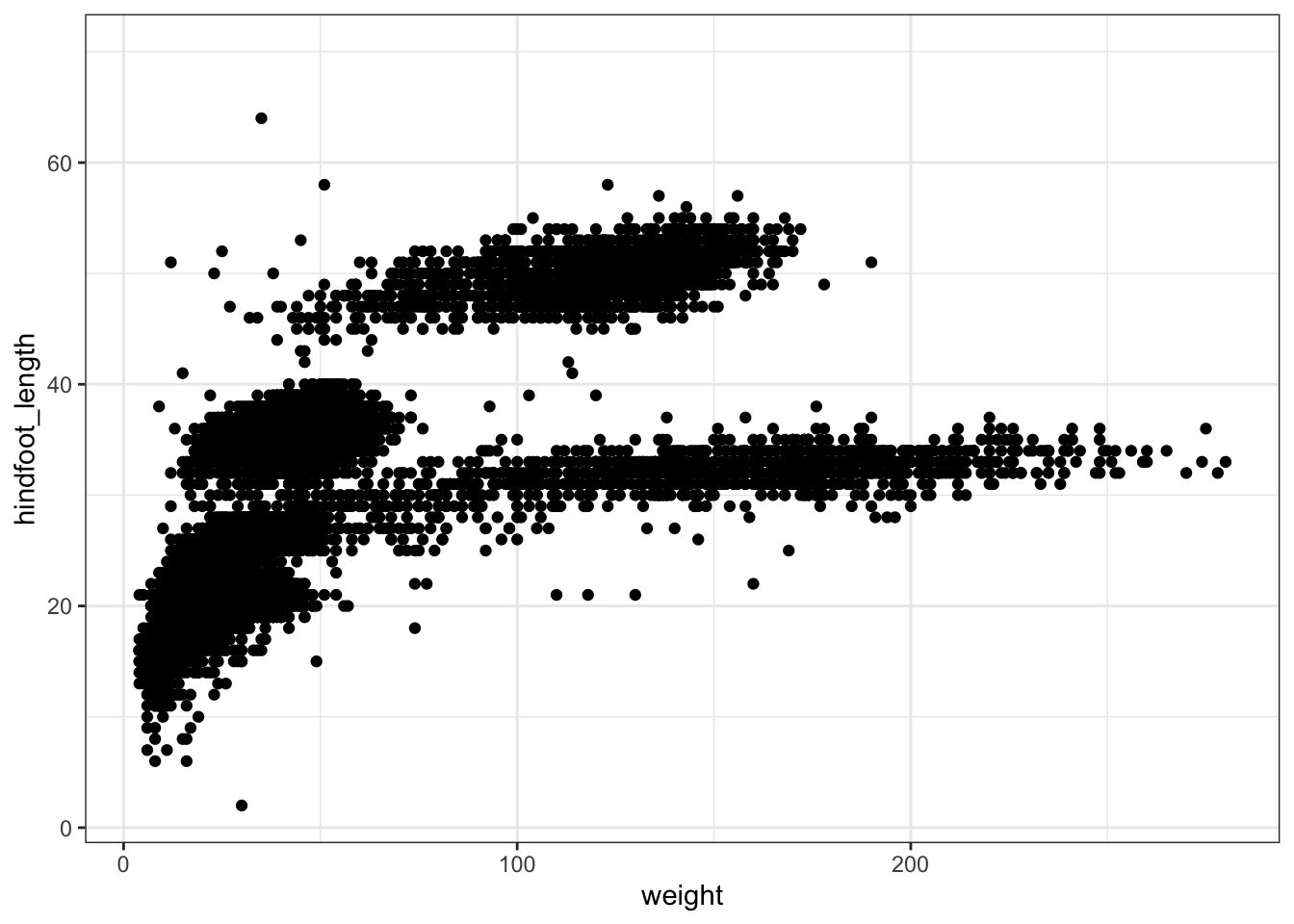
A list of themes can be found in the ggplot2 documentation.
Exercise 15
Level:
Using the surveys_complete variable, use what you just learned to create a plot that depicts how the average weight of each species changes through the years.
Solution for Exercise 15
surveys_complete %>%
  group_by(year, species) %>%
  summarize(avg_weight = mean(weight)) %>%
  ggplot(mapping = aes(x=year, y=avg_weight)) +
    geom_line() +
    facet_wrap(vars(species)) +
    theme_bw() +
    theme(axis.text.x = element_text(angle=90, vjust=0.5))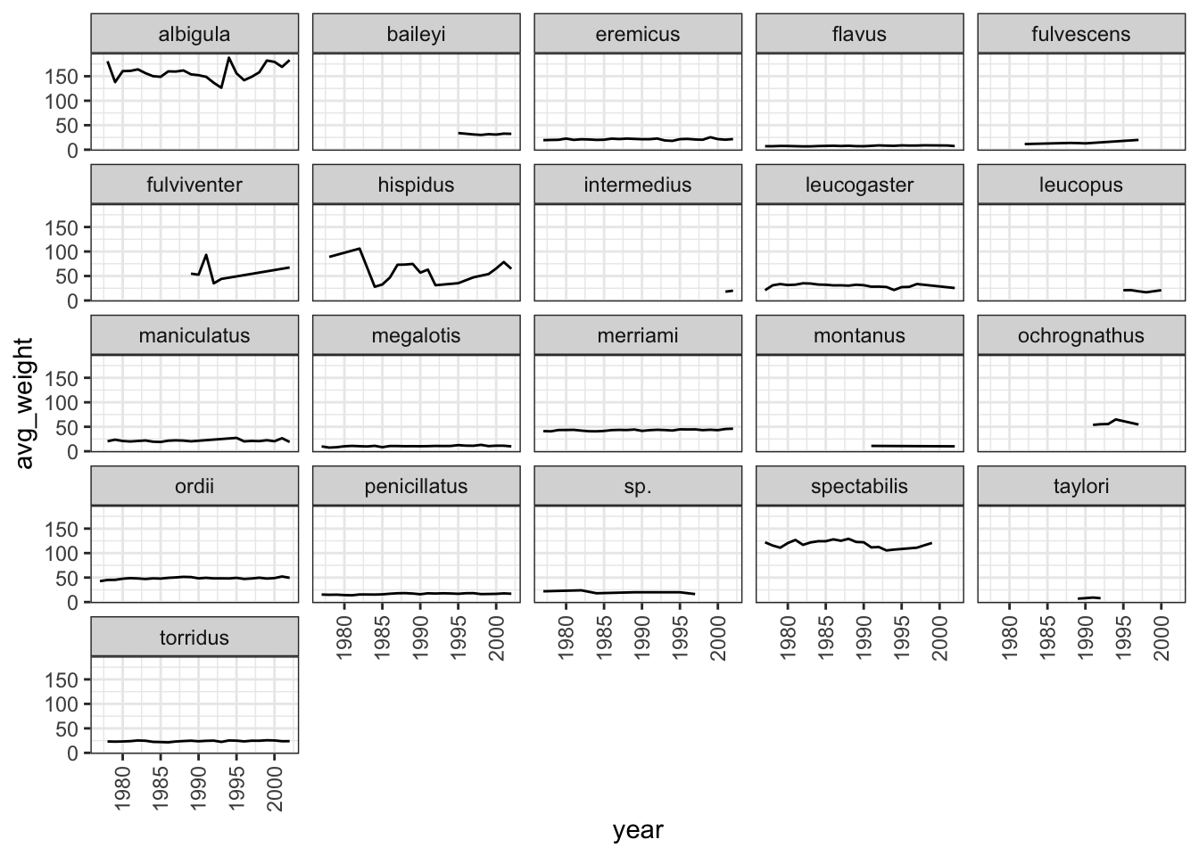
5.7 Exporting/Writing data to files
Now that you have learned how to use dplyr to transform your raw data, you may want to export these new datasets to share them with your collaborators or for archival.
Similar to the read_csv function used for reading CSV files into R, there is a write_csv function that generates CSV files from data frames and tibbles which is also present in the readr package.
Before using write_csv(), we are going to create a new folder, data_output, in our working directory that will store this generated dataset. We don’t want to write generated datasets in the same directory as our raw data. It’s good practice to keep them separate. The data folder should only contain the raw, unaltered data, and should be left alone to make sure we don’t delete or modify it. In contrast, our script will generate the contents of the data_output directory, so even if the files it contains are deleted, we can always re-generate them.
Let us save the surveys_complete tibble in data_output/surveys_complete.csv file:
write_csv(surveys_complete, file = "data_output/surveys_complete.csv")